
|
Tutorial Configuration Environment managment Graph managment Rules managment Execution managment |
This introduction consists in explaining how to use GPaR by developing a concrete project.
we consider the problem of adaptive mesh refinement for curve approximation.
Adaptive mesh refinement consists in creating iteratively new partitions of the considered space.
Individual grid cells is selected for refinement if some conditions are satisfied.
In this tutorial, triangle refinement is considered and the aim is to localize implicit functions defined by an equation depending on two variables x and y, namely f(x,y)=0.
The attribute AN=(cN,xN,yN) on nodes N consists in the xy-coordinates of N, xN and yN and a boolean cN equal to f(xN,yN)≤ 0:
There is no needs of attributes on ports. By default the position of the ports is computed automatically.
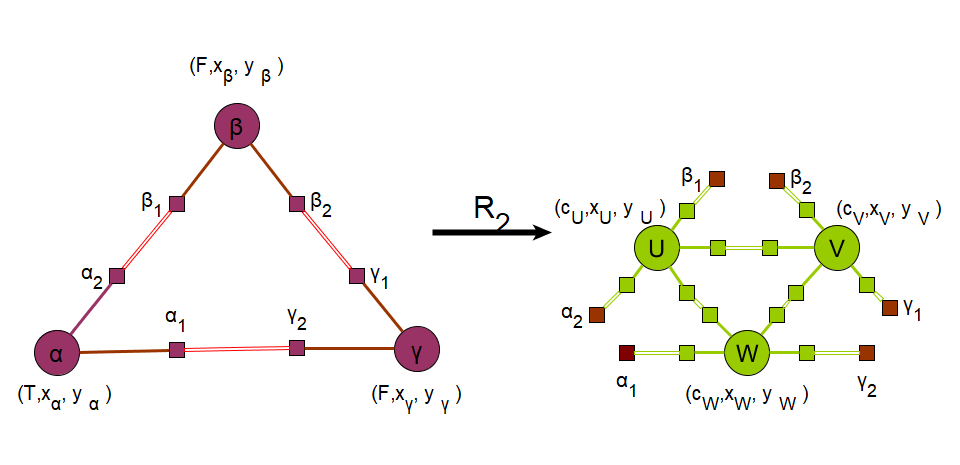
The refinement must be applied only on the triangles containing implicit functions of f(x,y)=0. A triangle will be decomposed into 4 triangles if the three c-attributes of the nodes defining the triangle are not equal. This constraint gives two rewriting rules depicted below.
In this drawing, big dots correspond to nodes and squares correspond to ports. The purple parts correspond to the environment parts. They allow to reconnect the new parts (in green) in the rewriting graph. The red parts correspond to the cut components. The environment part of the right-hand side must be included in the environment part of the left-hand side. It corresponds to the part needed to reconnect the new part in the rewritten graph. The environment part of the right-hand side cannot be removed by the action of an other rule, whereas the environment part of the left-hand side can be removed by the action of an other rule. In these specific example, nodes α, β and γ of the left-hand side are useful to compute the attributes of the new nodes U, V and W. For both rules : xU= (xα+xβ)/2, yU= (yα+yβ)/2, cU==(f(xU,yW) ≤ 0). xV= (xγ+xβ)/2, yV= (yγ+yβ)/2, cV==(f(xV,yV) ≤ 0), xW= (xα+xγ)/2, yW= (yα+yγ)/2, cW==(f(xW,yW) ≤ 0). Step by step, we will see how this problem can be modeled and implemented in GPaR. Successively, we will fill in
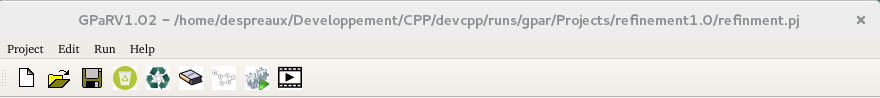
Once GPaR is launched, the following window appears:
Create your project by click on icon To configure the option of the soft, the preferences window can de edited by clicking on Edit->Preferences item. See the preferences section. To define the bivariate function f, click on the global environment button .
The following window appears: .
The following window appears:
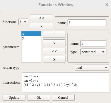
To add f as a global function, click on the ... button in the Global Functions area to make appear the Functions Window:
To declare the function, it is necessary to define:
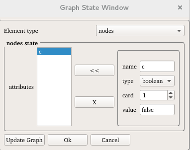
The next step consists in defining the attributes of the elements of the graph which can be either a node, a port or an edge.
Click on the button
In this window, select the graph element type whose state has to be defined and set the name, type, cardinality and default value of the new attribute. By default, positions of ports and nodes are already defined as attributes. Thus, in our example, we only have to add the node attribute c. The boxes have been filled in the following way :
 .
The Update Graph button allows to save all the modifications made in the graph state window,
otherwise all the modifications are not taken into account.
For more explanation about the graph state window, see the Attribute managment subsection. .
The Update Graph button allows to save all the modifications made in the graph state window,
otherwise all the modifications are not taken into account.
For more explanation about the graph state window, see the Attribute managment subsection.
The next step is to define the rewriting rule.
To do so, click on the button
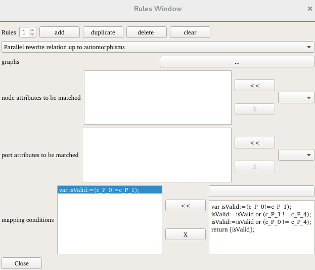
The first row indicates the rule index of the rule printed in the window. The 4 buttons are :
The option parallel rewrite relation up to automorphisms must be chosen in order to prevent several matches on each triangles. In this example, at most one match is applied per triangle. To define the graphs which corresponds to a rule, click on the ... button. The Rule Graph Window appears
 in the menu panel under the tool bar.
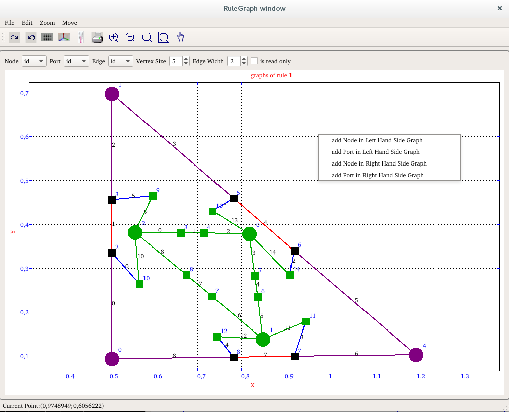
To add a vertex ( a node or a port) , put the mouse's pointer on the point on the drawing area where you want to create the vertex and click on the right button of the mouse to make appear the popup menu: Select the wanted item to add a vertex either in the left-hand side or in the right-hand side of the rule. Note that the two parts of the rule are defined in a single frame. The nodes and ports of the environment part which occurs in both the right and the left hand sides are considered as parts of the left-hand side with a specific label (see below for further explanations). All vertices have an Id which are defined automatically by GPaR. If a vertex of Id i belongs to the left-hand side, its label will be P_i, whereas if a vertex of Id i belongs to the right-hand side, its label will be T_i. To create an edge between two vertices, put the mouse's pointer on one of the two vertices and click on the right button of the mouse to make appear the popup menu : 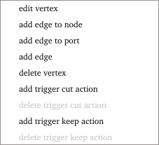 . .Select the wanted item and maintain the button pushed.
Note that a correct graph is a graph which verifies:
If an edge is added between 2 nodes, 2 ports are automatically created. If the connection is impossible, an error message appears.
To define the rewriting rules, create first the triangle of the left-hand side. In this tutorial, the nodes of the triangle are named P_0, P_1, P_4 and the ports are named P_2, P_3, P_5, P_6, P_7, P_8.
Graphically, the nodes are represented by dotes and the ports by squares. The size of those objects can be modified by using the menu panel under the tool bar. The color of the left-hand side is purple but again, this specification can be modified in the preference menu.
Now create the right-hand side by creating the nodes T_0, T_1, T_2 and the ports T_3, T_4, T_5, T_6, T_7, T_8, T_9, T_10, T_11, T_12, T_13, T_14.
The subgraph supported by those vertices is represented in green.
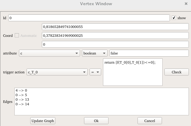
To connect the purple graph with the green graph which corresponds to the new part of the right-hand side of the rewriting rule, the edges (T_9,P_3), (T_10,P_2), (T_11,P_7), (T_12,P_8), (T_13,P_5), (T_14,P_6) have to be added. For instance, the coordinates of the node T_0 must be at the middle of the segment [P_1,P_4] : put the mouse pointer on the node T_0 and select the edit vertex after clicking on the right button of the mouse to make appear the popup menu or click twice on the node T_0. The following window appears:
In this window, appear from top to bottom:
The trigger action corresponds to the function which has to be applied on state. In this tutorial, we want to return the boolean value corresponding to true if the implicit function at the point is negative. it can be translated as follow: return [f(T_0[0],T_0[1])<=0];
T_0 is the point of the new part with id 0, T_0[i] is the i-coordinate value of the point. To set the coordinates of T_0, select T_0 on the combo box selection after trigger action, and set the point to the middle of segment [P_1,P_4], translated as follow: return [0.5*(P_1+P_4)];For more explanations on setting rules on state of window see the state managment subsection. For more explanations on the syntax of algebraic formula, see the math formula parser subsection. Proceed in the same way for the nodes T_1 and T_2. Remark that the state of the vertices of the left-hand side can also be modified. In this case the compatibility of the state vertices is checked during the reconstruction of the rewritten graph. If a attribute vertex has 2 different values, a error message appear. Having decided on the rule and the states of new elements, we must decide the conditions of matches. This has to be done in the Rules Window.
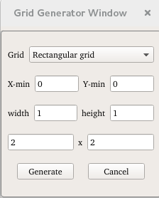
 of the main window. of the main window.We would like to generate a grid in the rectangle [-2,2] × [-2,2] of the 2D-plane. We can do it by hands but we can use the generate grid item of the edit menu of the graph window:
Choose the isosceles triangular mesh to obtain the following grid:
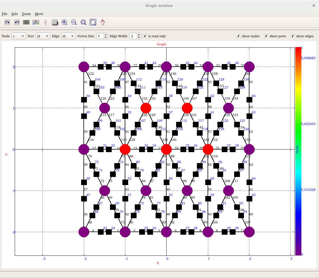
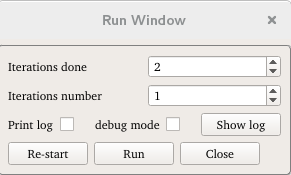
The initial value of the state of the graph's element can be setting by double clicked on the graph element. Its graph element window appears and it is easy to set the value of the attributes of the state. Here, we see in red the nodes whose the c attribute is true and in purple, the nodes whose c attribute is false. It is possible to show the value of the state of a graph element (node, port or edge) by selecting the corresponding state we want to show. Here we have selected the c attribute of node, the id of ports and edges. For more explanations on this window, see the graph managment section. The parallel application of a set of rules rewrite an initial graph named g0 into a new graph named g1 in one step. In the example of mesh refinement, several parallel iterations are needed in order to obtain a precise approximation of the implicit curve of f(x,y)=0. At the second iteration, g1 is rewritten into g2, etc) To perform the parallel graph rewriting process on the initial graph, click on the execute  button, the Run Window appears. button, the Run Window appears.
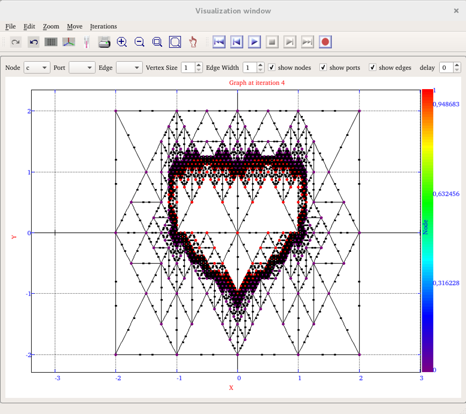
The movie window enables to see the graph evolution over the iterations. It is possible to print the value of the state of nodes, ports or edges by selecting the states to show from the bar 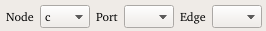 and to choose the width for vertices and edges representation as line or disk from the bar
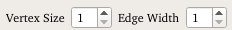 . .It is also possible to show (or mask) nodes, ports or edges and to adjust the delay between two iterations in seconds from the tool bar  . .For more explanations, see the Execution managment section. |

 ,
or select Project in the menu of the main
window and select New Project. See the
,
or select Project in the menu of the main
window and select New Project. See the 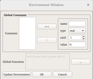
 to define the attributes of the elements of the graph.
 to show the rule window.